My PyTorch implementation for tensor decomposition methods on convolutional layers.
Notebook contributed to TensorLy.
Background
In this post I will cover a few low rank tensor decomposition methods for taking layers in existing deep learning models and making them more compact. I will also share PyTorch code that uses Tensorly for performing CP decomposition and Tucker decomposition of convolutional layers.
Although hopefully most of the post is self contained, a good review of tensor decompositions can be found here. The author of Tensorly also created some really nice notebooks about Tensors basics. That helped me getting started, and I recommend going through that.
Together with pruning, tensor decompositions are practical tools for speeding up existing deep neural networks, and I hope this post will make them a bit more accessible.
These methods take a layer and decompose it into several smaller layers. Although there will be more layers after the decomposition, the total number of floating point operations and weights will be smaller. Some reported results are on the order of x8 for entire networks (not aimed at large tasks like imagenet, though), or x4 for specific layers inside imagenet. My experience was that with these decompositions I was able to get a speedup of between x2 to x4, depending on the accuracy drop I was willing to take.
In this blog post I covered a technique called pruning for reducing the number of parameters in a model. Pruning requires making a forward pass (and sometimes a backward pass) on a dataset, and then ranks the neurons according to some criterion on the activations in the network.
Quite different from that, tensor decomposition methods use only the weights of a layer, with the assumption that the layer is over parameterized and its weights can be represented by a matrix or tensor with a lower rank. This means they work best in cases of over parameterized networks. Networks like VGG are over parameterized by design. Another example of an over parameterized model is fine tuning a network for an easier task with fewer categories.
Similarly to pruning, after the decomposition usually the model needs to be fine tuned to restore accuracy.
One last thing worth noting before we dive into details, is that while these methods are practical and give nice results, they have a few drawbacks:
- They operate on the weights of a linear layer (like a convolution or a fully connected layer), and ignore any non linearity that comes after them.
- They are greedy and perform the decomposition layer wise, ignoring interactions between different layers.
There are works that try to address these issues, and its still an active research area.
Truncated SVD for decomposing fully connected layers
The first reference I could find of using this for accelerating deep neural networks, is in the Fast-RCNN paper. Ross Girshick used it to speed up the fully connected layers used for detection. Code for this can be found in the pyfaster-rcnn implementation.
SVD recap
The singular value decomposition lets us decompose any matrix A with n rows and m columns:
\[A_{nxm} = U_{nxn} S_{nxm} V^T_{mxm}\]S is a diagonal matrix with non negative values along its diagonal (the singular values), and is usually constructed such that the singular values are sorted in descending order. U and V are orthogonal matrices: \(U^TU=V^TV=I\)
If we take the largest t singular values and zero out the rest, we get an approximation of A: \(\hat{A} = U_{nxt}S_{txt}V^T_{mxt}\)
\(\hat{A}\) has the nice property of being the rank t matrix that has the Frobenius-norm closest to A, so \(\hat{A}\) is a good approximation of A if t is large enough.
SVD on a fully connected layer
A fully connected layer essentially does matrix multiplication of its input by a matrix A, and then adds a bias b:
\(Ax+b\).
We can take the SVD of A, and keep only the first t singular values.
\((U_{nxt}S_{txt}V^T_{mxt})x + b\) = \(U_{nxt} ( S_{txt}V^T_{mxt} x ) + b\)
Instead of a single fully connected layer, this guides us how to implement it as two smaller ones:
- The first one will have a shape of mxt, will have no bias, and its weights will be taken from \(S_{txt}V^T\).
- The second one will have a shape of txn, will have a bias equal to b, and its weights will be taken from \(U\).
The total number of weights dropped from nxm to t(n+m).
Tensor decompositions on convolutional layers
A 2D convolutional layer is a multi dimensional matrix (from now on - tensor) with 4 dimensions:
cols x rows x input_channels x output_channels.
Following the SVD example, we would want to somehow decompose the tensor into several smaller tensors. The convolutional layer would then be approximated by several smaller convolutional layers.
For this we will use the two popular (well, at least in the world of Tensor algorithms) tensor decompositions: the CP decomposition and the Tucker decomposition (also called higher-order SVD and many other names).
1412.6553 Speeding-up Convolutional Neural Networks Using Fine-tuned CP-Decomposition
1412.6553 Speeding-up Convolutional Neural Networks Using Fine-tuned CP-Decomposition shows how CP-Decomposition can be used to speed up convolutional layers. As we will see, this factors the convolutional layer into something that resembles mobile nets.
They were able to use this to accelerate a network by more than x8 without significant decrease in accuracy. In my own experiments I was able to use this get a x2 speedup on a network based on VGG16 without accuracy drop.
My experience with this method is that the finetuning learning rate needs to be chosen very carefuly to get it to work, and the learning rate should usually be very small (around \(10^{-6}\)).
A rank R matrix can be viewed as a sum of R rank 1 matrices, were each rank 1 matrix is a column vector multiplying a row vector: \(\sum_1^Ra_i*b_i^T\)
The SVD gives us a way for writing this sum for matrices using the columns of U and V from the SVD: \(\sum_1^R \sigma_i u_i*v_i^T\).
If we choose an R that is less than the full rank of the matrix, than this sum is just an approximation, like in the case of truncated SVD.
The CP decomposition lets us generalize this for tensors.
Using CP-Decompoisition, our convolutional kernel, a 4 dimensional tensor \(K(i, j, s, t)\) can be approximated similarly for a chosen R:
\(\sum_{r=1}^R K^x_r(i)K^y_r(j)K^s_r(s)K^t_r(t)\).
We will want R to be small for the decomposition to be effecient, but large enough to keep a high approximation accuracy.
The convolution forward pass with CP Decomposition
To forward the layer, we do convolution with an input \(X(i, j, s)\):
\(V(x, y, t) = \sum_i \sum_j \sum_sK(i, j, s, t)X(x-i, y-j, s)\) \(= \sum_r\sum_i \sum_j \sum_sK^x_r(i)K^y_r(i)K^s_r(s)K^t_r(t)X(x-i, y-j, s)\) \(= \sum_rK^t_r(t) \sum_i \sum_j K^x_r(i)K^y_r(i)\sum_sK^s_r(s)X(x-i, y-j, s)\)
This gives us a recipe to do the convlution:
-
First do a point wise (1x1xS) convolution with \(K_r(s)\). This reduces the number of input channels from S to R. The convolutions will next be done on a smaller number of channels, making them faster.
-
Perform seperable convolutions in the spatial dimensions with \(K^x_r,K^y_r\). Like in mobilenets the convolutions are depthwise seperable, done in each channel separately. Unlike mobilenets the convolutions are also separable in the spatial dimensions.
-
Do another pointwise convolution to change the number of channels from R to T If the original convolutional layer had a bias, add it at this point.
Notice the combination of pointwise and depthwise convolutions like in mobilenets. While with mobilenets you have to train a network from scratch to get this structure, here we can decompose an existing layer into this form.
As with mobile nets, to get the most speedup you will need a platform that has an efficient implementation of depthwise separable convolutions.
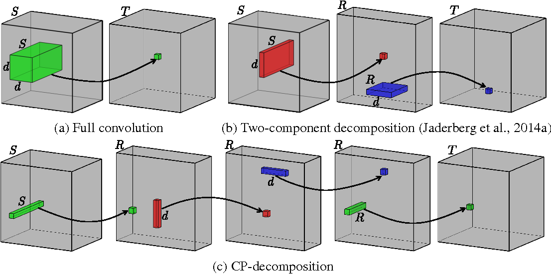 Image taken from the paper. The bottom row is an illustration of the convolution steps after CP-decomposition.
Convolutional layer CP-Decomposition with PyTorch and Tensorly
def cp_decomposition_conv_layer(layer, rank):
    """ Gets a conv layer and a target rank,
        returns a nn.Sequential object with the decomposition """

    # Perform CP decomposition on the layer weight tensorly.
    last, first, vertical, horizontal = \
        parafac(layer.weight.data, rank=rank, init='svd')

    pointwise_s_to_r_layer = torch.nn.Conv2d(in_channels=first.shape[0], \
            out_channels=first.shape[1], kernel_size=1, stride=1, padding=0,
            dilation=layer.dilation, bias=False)

    depthwise_vertical_layer = torch.nn.Conv2d(in_channels=vertical.shape[1],
            out_channels=vertical.shape[1], kernel_size=(vertical.shape[0], 1),
            stride=1, padding=(layer.padding[0], 0), dilation=layer.dilation,
            groups=vertical.shape[1], bias=False)

    depthwise_horizontal_layer = \
        torch.nn.Conv2d(in_channels=horizontal.shape[1], \
            out_channels=horizontal.shape[1],
            kernel_size=(1, horizontal.shape[0]), stride=layer.stride,
            padding=(0, layer.padding[0]),
            dilation=layer.dilation, groups=horizontal.shape[1], bias=False)

    pointwise_r_to_t_layer = torch.nn.Conv2d(in_channels=last.shape[1], \
            out_channels=last.shape[0], kernel_size=1, stride=1,
            padding=0, dilation=layer.dilation, bias=True)

    pointwise_r_to_t_layer.bias.data = layer.bias.data

    depthwise_horizontal_layer.weight.data = \
        torch.transpose(horizontal, 1, 0).unsqueeze(1).unsqueeze(1)
    depthwise_vertical_layer.weight.data = \
        torch.transpose(vertical, 1, 0).unsqueeze(1).unsqueeze(-1)
    pointwise_s_to_r_layer.weight.data = \
        torch.transpose(first, 1, 0).unsqueeze(-1).unsqueeze(-1)
    pointwise_r_to_t_layer.weight.data = last.unsqueeze(-1).unsqueeze(-1)

    new_layers = [pointwise_s_to_r_layer, depthwise_vertical_layer, \
                    depthwise_horizontal_layer, pointwise_r_to_t_layer]

    return nn.Sequential(*new_layers)
1511.06530 Compression of Deep Convolutional Neural Networks for Fast and Low Power Mobile Applications
1511.06530 Compression of Deep Convolutional Neural Networks for Fast and Low Power Mobile Applications is a really cool paper that shows how to use the Tucker Decomposition for speeding up convolutional layers with even better results. I also used this accelerate an over-parameterized VGG based network, with better accuracy than CP Decomposition. As the authors note in the paper, it lets us do the finetuning using higher learning rates (I used \(10^{-3}\)).
The Tucker Decomposition, also known as the higher order SVD (HOSVD) and many other names, is a generalization of SVD for tensors. \(K(i, j, s, t) = \sum_{r_1=1}^{R_1}\sum_{r_2=1}^{R_2}\sum_{r_3=1}^{R_3}\sum_{r_4=1}^{R_4}\sigma_{r_1 r_2 r_3 r_4} K^x_{r1}(i)K^y_{r2}(j)K^s_{r3}(s)K^t_{r4}(t)\)
The reason its considered a generalization of the SVD is that often the components of \(\sigma_{r_1 r_2 r_3 r_4}\) are orthogonal, but this isn’t really important for our purpose. \(\sigma_{r_1 r_2 r_3 r_4}\) is called the core matrix, and defines how different axis interact.
In the CP Decomposition described above, the decomposition along the spatial dimensions \(K^x_r(i)K^y_r(j)\) caused a spatially separable convolution. The filters are quite small anyway, typically 3x3 or 5x5, so the separable convolution isn’t saving us a lot of computation, and is an aggressive approximation.
The Tucker decomposition has the useful property that it doesn’t have to be decomposed along all the axis (modes). We can perform the decomposition along the input and output channels instead (a mode-2 decomposition):
\[K(i, j, s, t) = \sum_{r_3=1}^{R_3}\sum_{r_4=1}^{R_4}\sigma_{i j r_3 r_4}(j)K^s_{r3}(s)K^t_{r4}(t)\]The convolution forward pass with Tucker Decomposition
Like for CP decomposition, lets write the convolution formula and plug in the kernel decomposition:
\[V(x, y, t) = \sum_i \sum_j \sum_sK(i, j, s, t)X(x-i, y-j, s)\] \[V(x, y, t) = \sum_i \sum_j \sum_s\sum_{r_3=1}^{R_3}\sum_{r_4=1}^{R_4}\sigma_{(i)(j) r_3 r_4}K^s_{r3}(s)K^t_{r4}(t)X(x-i, y-j, s)\] \[V(x, y, t) = \sum_i \sum_j \sum_{r_4=1}^{R_4}\sum_{r_3=1}^{R_3}K^t_{r4}(t)\sigma_{(i)(j) r_3 r_4} \sum_s\ K^s_{r3}(s)X(x-i, y-j, s)\]This gives us the following recipe for doing the convolution with Tucker Decomposition:
-
Point wise convolution with \(K^s_{r3}(s)\) for reducing the number of channels from S to \(R_3\).
-
Regular (not separable) convolution with \(\sigma_{(i)(j) r_3 r_4}\). Instead of S input channels and T output channels like the original layer had, this convolution has \(R_3\) input channels and \(R_4\) output channels. If these ranks are smaller than S and T, this is were the reduction comes from.
-
Pointwise convolution with \(K^t_{r4}(t)\) to get back to T output channels like the original convolution. Since this is the last convolution, at this point we add the bias if there is one.
How can we select the ranks for the decomposition ?
One way would be trying different values and checking the accuracy. I played with heuristics like \(R_3 = S/3\) , \(R_4 = T/3\) with good results.
Ideally selecting the ranks should be automated.
The authors suggested using variational Bayesian matrix factorization (VBMF) (Nakajima et al., 2013) as a method for estimating the rank.
VBMF is complicated and is out of the scope of this post, but in a really high level summary what they do is approximate a matrix \(V_{LxM}\) as the sum of a lower ranking matrix \(B_{LxH}A^T_{HxM}\) and gaussian noise. After A and B are found, H is an upper bound on the rank.
To use this for tucker decomposition, we can unfold the s and t components of the original weight tensor to create matrices. Then we can estimate \(R_3\) and \(R_4\) as the rank of the matrices using VBMF.
I used this python implementation of VBMF and got convinced it works :-)
VBMF usually returned ranks very close to what I previously found with careful and tedious manual tuning.
This could also be used for estimating the rank for Truncated SVD acceleration of fully connected layers.
Convolutional layer Tucker-Decomposition with PyTorch and Tensorly
def estimate_ranks(layer):
    """ Unfold the 2 modes of the Tensor the decomposition will
    be performed on, and estimates the ranks of the matrices using VBMF
    """

    weights = layer.weight.data.numpy()
    unfold_0 = tensorly.base.unfold(weights, 0)
    unfold_1 = tensorly.base.unfold(weights, 1)
    _, diag_0, _, _ = VBMF.EVBMF(unfold_0)
    _, diag_1, _, _ = VBMF.EVBMF(unfold_1)
    ranks = [diag_0.shape[0], diag_1.shape[1]]
    return ranks

def tucker_decomposition_conv_layer(layer):
    """ Gets a conv layer,
        returns a nn.Sequential object with the Tucker decomposition.
        The ranks are estimated with a Python implementation of VBMF
        https://github.com/CasvandenBogaard/VBMF
    """

    ranks = estimate_ranks(layer)
    print(layer, "VBMF Estimated ranks", ranks)
    core, [last, first] = \
        partial_tucker(layer.weight.data, \
            modes=[0, 1], ranks=ranks, init='svd')

    # A pointwise convolution that reduces the channels from S to R3
    first_layer = torch.nn.Conv2d(in_channels=first.shape[0], \
            out_channels=first.shape[1], kernel_size=1,
            stride=1, padding=0, dilation=layer.dilation, bias=False)

    # A regular 2D convolution layer with R3 input channels
    # and R3 output channels
    core_layer = torch.nn.Conv2d(in_channels=core.shape[1], \
            out_channels=core.shape[0], kernel_size=layer.kernel_size,
            stride=layer.stride, padding=layer.padding, dilation=layer.dilation,
            bias=False)

    # A pointwise convolution that increases the channels from R4 to T
    last_layer = torch.nn.Conv2d(in_channels=last.shape[1], \
        out_channels=last.shape[0], kernel_size=1, stride=1,
        padding=0, dilation=layer.dilation, bias=True)

    last_layer.bias.data = layer.bias.data

    first_layer.weight.data = \
        torch.transpose(first, 1, 0).unsqueeze(-1).unsqueeze(-1)
    last_layer.weight.data = last.unsqueeze(-1).unsqueeze(-1)
    core_layer.weight.data = core

    new_layers = [first_layer, core_layer, last_layer]
    return nn.Sequential(*new_layers)
Summary
In this post we went over a few tensor decomposition methods for accelerating layers in deep neural networks.
-
Truncated SVD can be used for accelerating fully connected layers.
-
CP Decomposition decomposes convolutional layers into something that resembles mobile-nets, although it is even more aggressive since it is also separable in the spatial dimensions.
-
Tucker Decomposition reduced the number of input and output channels the 2D convolution layer operated on, and used pointwise convolutions to switch the number of channels before and after the 2D convolution.
I think it’s interesting how common patterns in network design, pointwise and depthwise convolutions, naturally appear in these decompositions!